4.14 Regression Lesson 14
Bear in mind, regression is a subject of the Supervised branch of Machine Learning. Figure 1 shows a simple big picture.

Some hot points in these two branches (there are other branches, but these two are the most know).
- Supervised: A machine learning technique where we are attempting to predict a label based on inputs.
- Predict fraudulent transactions
- Predict chance of default on a loan
- Predict home prices
- Unsupervised: A machine learning technique where we are attempting to group together unlabeled data based on similar characteristics.
- Customer segmentation
- Group document that cover similar topics
The Linear and Logistic Regression fall into the Supervised Machine Learning branch.
4.14.1 Introduction to Linear Regression
- Response variable or dependent (y): The variable you are interested in predicting, and;
- Explanatory variable or independent (x): The variable used to predicted the response.
A common way to visualize the relationship between two variables in linear regression is using a scatterplot. You will see more on this in the concepts ahead. — Udacity notebook
Figure 2 shows an example of a scatter plot.
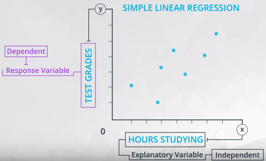
4.14.1.1 Scatter Plot
Scatter plots are a common visual for comparing two quantitative variables. A common summary statistic that relates to a scatter plot is the correlation coefficient commonly denoted by
r.Though there are a few different ways to measure correlation between two variables, the most common way is with Pearson’s correlation coefficient. Pearson’s correlation coefficient provides the:
- Strength
- Direction
of a linear relationship. Spearman’s Correlation Coefficient does not measure linear relationships specifically, and it might be more appropriate for certain cases of associating two variables. — Udacity notebook
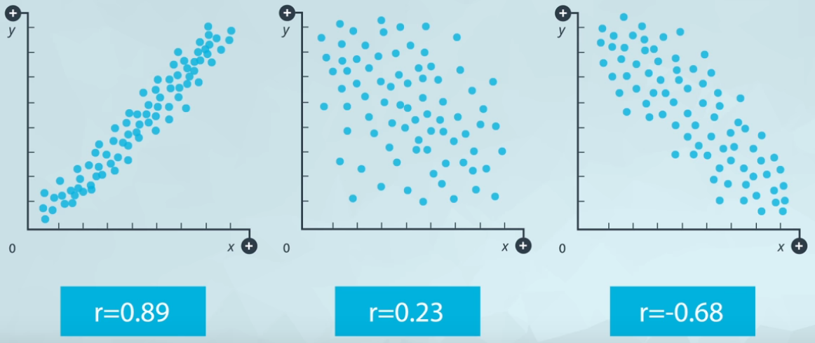
Figure 3 shows an example of strong positive relationship.
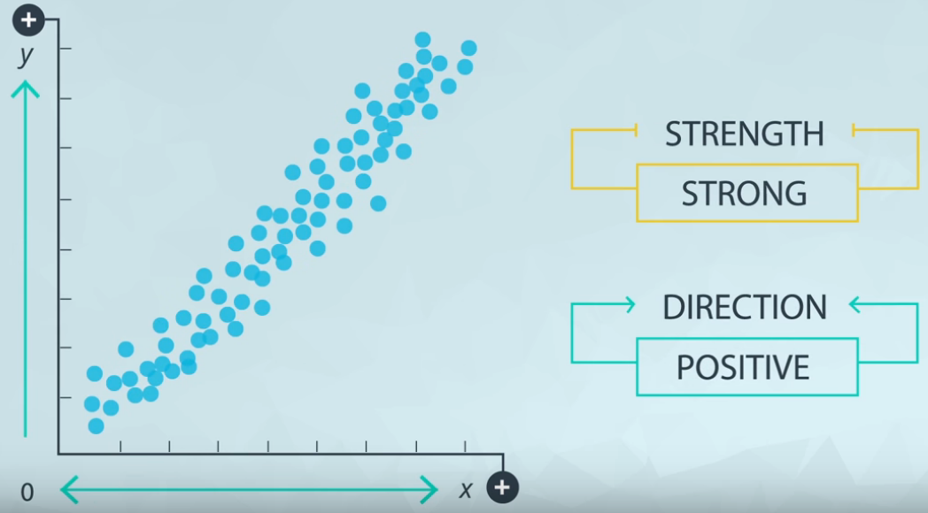
When x increase y also increase, and the points is very close from each other. Figure 4 shows the opposite of positive direction.
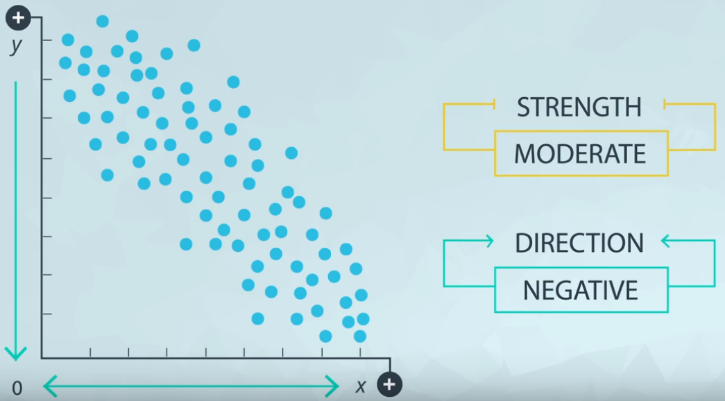
When x increase y decrease, and the points is a bit sparse. Figure 5 shows an example of scatter plot with weak strength.
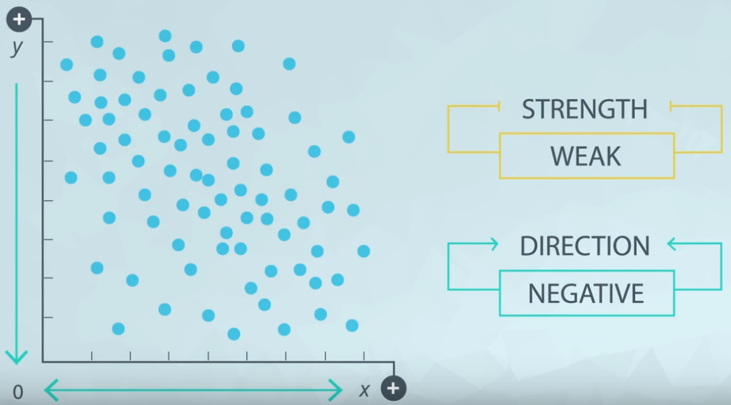
Both, strength and direction is capture by the correlation (r).
- Correlation
- Varies from -1 to +1;
- Values close to -1 and +1 are very strong;
- The signal (positive or negative) means the direction.
4.14.2 Correlation Coefficients
This is highly field-dependent measure and these values are a general rule of thumbs.
Have in mind, in social sciences is very difficult to find a strong correlation (probably because human are very complex and hard to understand).
- Strong: \(0.7 \leq |r| \leq 1.0\)
- Moderate: \(0.3 \leq |r| \leq .7\)
- Weak: \(0.0 \leq |r| \leq 0.3\)
Sometimes a plot could help a lot, Figure 7 shows an example of two graphs with same correlation coefficients.

This problem presented in Figure 6 is part of the Anscombe’s Quartet images.
4.14.3 Coefficients
A Linear Regression is a way to estimate the values of some coefficients:
- Intercept: The expected value of the response when the explanatory variable is 0 (zero);
- \(b_0:\) statistic value (sample)
- \(\beta_0:\) parameter value (population)
- Slope: The expected change in the response for each 1 unit increase in the explanatory variable.
- \(b_1:\) statistic value (sample)
- \(\beta_1:\) parameter value (population)
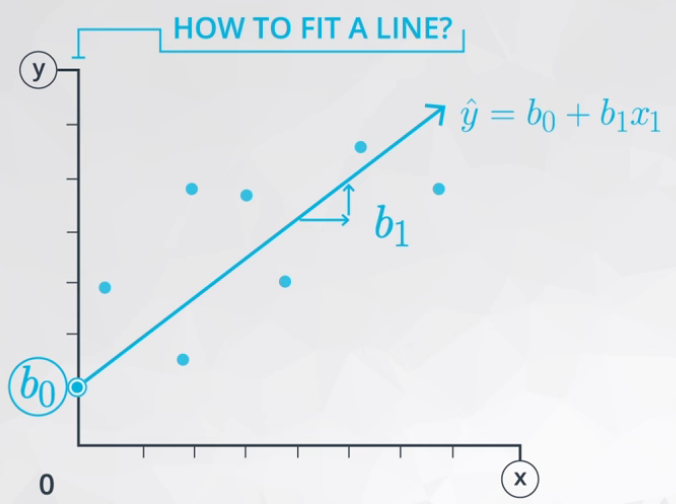
Based on the Intercept and Slope, the Linear Regression equation is presented in equation (1).
\[ \hat y = b_0 + b_1x \]
Where: * \(\hat y:\) is the predicted value of the response from the line. * \(y:\) is an actual response value for a data point in our dataset (not a prediction from our line). * \(b_0:\) is the intercept. * \(b_1:\) is the slope. * \(x_1:\) is the explanatory variable.
Figure 8 ilustrate this equation in a picture.
4.14.4 Least-squares
A work by AH Uyekita
anderson.uyekita[at]gmail.com