4.4 Probability Lesson 04
4.4.1 Introduction to Probability
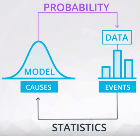
Do not confound Statistics and Probability.
- Probability: Make preditcions about the future events based on models, and;
- Here I want to predict data!
- Statistics: Analyze data from past events to infer what those models or causes could be.
- Here I use data to preditc!
Figure 1 shows the relation between these two subjects.

4.4.1.1 Fair Coin
The probability notation is based on the 0 to 1 scale, where 0 means zero percentage and 1 means 100 percentage. The example below is a 50%.
\[ P(HEADS) = 0.5 \]
To be a fair coin the tail probability it is the same of heads.
\[ P(TAILS) = 0.5 \]
4.4.1.2 Loaded Coin
Its occurs when the \(P(HEADS)\) is different of \(P(TAILS)\). Bear in mind, in the equation 1.
\[ P(HEADS) + P(TAILS) = 1 \tag{1}\]
Example 1: {HEADS, HEADS} = \(P(H, H)\) for a fair coin.
\(P(H) = P(T) = 0.5\)
To ilustrate this solution, let’s draw the Truth Table (Table 1)
| Flip 1 | Flip 2 | Probability |
|---|---|---|
| H | H | $ 0.5 * 0.5 = 0.25 $ |
| H | T | $ 0.5 * 0.5 = 0.25 $ |
| T | H | $ 0.5 * 0.5 = 0.25 $ |
| T | T | $ 0.5 * 0.5 = 0.25 $ |
| $ SUM = 1.0 $ |
The probability of P(H, H) is 0.25.
Example 2: {HEADS, HEADS} = \(P(H, H)\) for a loaded coin.
$ P(H) = 0.6 $ $ P(T) = 0.4 $
To ilustrate this solution, let’s draw the Truth Table (Table 2)
| Flip 1 | Flip 2 | Probability |
|---|---|---|
| H | H | $ 0.6 * 0.6 = 0.36 $ |
| H | T | $ 0.6 * 0.4 = 0.24 $ |
| T | H | $ 0.4 * 0.6 = 0.24 $ |
| T | T | $ 0.4 * 0.4 = 0.16 $ |
| $ SUM = 1.0 $ |
The probability of P(H, H) is 0.36.
Example 3: Three coins flipped. What is the probability of only one heads in three coins flipped. Adopting a fair coin ($ P(H) = 0.5 $).
\(P_1(Only one H)\)
| Flip 1 | Flip 2 | Flip 3 | Probability | Has only one heads? | \(P_1\) |
|---|---|---|---|---|---|
| H | H | H | $ 0.5 * 0.5 * 0.5 = 0.125 $ | No | 0 |
| H | H | T | $ 0.5 * 0.5 * 0.5 = 0.125 $ | No | 0 |
| H | T | H | $ 0.5 * 0.5 * 0.5 = 0.125 $ | No | 0 |
| H | T | T | $ 0.5 * 0.5 * 0.5 = 0.125 $ | Yes | 0.125 |
| T | H | H | $ 0.5 * 0.5 * 0.5 = 0.125 $ | No | 0 |
| T | H | T | $ 0.5 * 0.5 * 0.5 = 0.125 $ | Yes | 0.125 |
| T | T | H | $ 0.5 * 0.5 * 0.5 = 0.125 $ | Yes | 0.125 |
| T | T | T | $ 0.5 * 0.5 * 0.5 = 0.125 $ | No | 0 |
| $ SUM = 1.0 $ | $ SUM = 3 $ | $ SUM = 0.375 $ |
The $ P_1 $ is 0.375.
Example 4: Three coins flipped. What is the probability of only one heads in three coins flipped. Adopting a loaded coin ($ P(H) = 0.6 $).
\(P_2(Only one H)\)
| Flip 1 | Flip 2 | Flip 3 | Probability | Has only one heads? | \(P_2\) |
|---|---|---|---|---|---|
| H | H | H | $ 0.6 * 0.6 * 0.6 = 0.216 $ | No | 0 |
| H | H | T | $ 0.6 * 0.6 * 0.4 = 0.144 $ | No | 0 |
| H | T | H | $ 0.6 * 0.4 * 0.6 = 0.144 $ | No | 0 |
| H | T | T | $ 0.6 * 0.4 * 0.4 = 0.096 $ | Yes | 0.096 |
| T | H | H | $ 0.4 * 0.6 * 0.6 = 0.144 $ | No | 0 |
| T | H | T | $ 0.4 * 0.6 * 0.4 = 0.096 $ | Yes | 0.096 |
| T | T | H | $ 0.4 * 0.4 * 0.6 = 0.096 $ | Yes | 0.096 |
| T | T | T | $ 0.4 * 0.4 * 0.4 = 0.064 $ | No | 0 |
| $ SUM = 1.0 $ | $ SUM = 3 $ | $ SUM = 0.288 $ |
The $ P_2 $ is 0.288.
4.4.2 Bernoulli Distribution
Founded on this introduction, let’s generalize this concept using the Bernoulli Distribution.
In probability theory and statistics, the Bernoulli distribution, named after Swiss mathematician Jacob Bernoulli, is the discrete probability distribution of a random variable which takes the value 1 with probability \({\displaystyle p}\) and the value 0 with probability \({\displaystyle q=1-p,}\) that is, the probability distribution of any single experiment that asks a yes–no question; the question results in a boolean-valued outcome, a single bit of information whose value is success/yes/true/one with probability p and failure/no/false/zero with probability q. It can be used to represent a (possibly biased) coin toss where 1 and 0 would represent “heads” and “tails” (or vice versa), respectively, and p would be the probability of the coin landing on heads or tails, respectively. In particular, unfair coins would have \({\displaystyle p\neq 1/2.}\)
The Bernoulli distribution is a special case of the binomial distribution where a single trial is conducted (so n would be 1 for such a binomial distribution). It is also a special case of the two-point distribution, for which the possible outcomes need not be 0 and 1. – Wikipedia
Rede more in wolfram.
4.4.2.1 Summary
Here you learned some fundamental rules of probability. Using notation, we could say that the outcome of a coin flip could either be T or H for the event that the coin flips tails or heads, respectively.
Then the following rules are true:
Probability of a Event > \[\bold{P(H)} = 0.5\]
Probability of opposite event > \[\bold{1 - P(H) = P(\text{not H})} = 0.5\]
where \(\bold{\text{not H}}\) is the event of anything other than heads. Since, there are only two possible outcomes, we have that \(\bold{P(\text{not H}) = P(T)} = 0.5\). In later concepts, you will see this with the following notation: \(\bold{\lnot H}\).
- Probability of composite event
\[ P * P * P * \dots * P \]
It is only true because the events are independent of one another, which means the outcome of one does not affect the outcome of another.
- Across multiple coin flips, we have the probability of seeing n heads as \(\bold{P(H)^n}\). This is because these events are independent.
We can get two generic rules from this:
- The probability of any event must be between 0 and 1, inclusive.
- The probability of the compliment event is 1 minus the probability of an event. That is the probability of all other possible events is 1 minus the probability an event itself. Therefore, the sum of all possible events is equal to 1.
- If our events are independent, then the probability of the string of possible events is the product of those events. That is the probability of one event AND the next AND the next event, is the product of those events.
4.4.2.2 Looking Ahead
You will be working with the Binomial Distribution, which creates a function for working with coin flip events like the first events in this lesson. These events are independent, and the above rules will hold. from Text: Recap + Next Steps
4.4.3 Conditional Probability
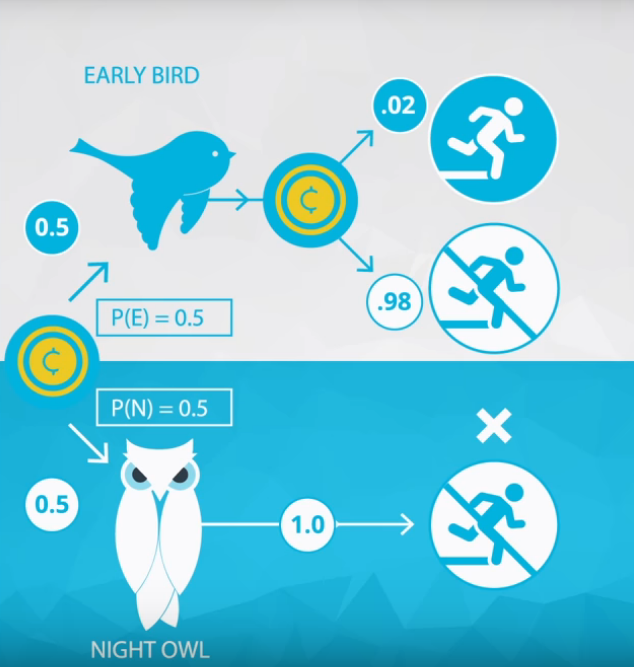
Here the first event will affect the second one. Figure 1 shows an example of it.

Figure 1
The first event is to determine the bird type, and the second event the probability to run on the morning. Have in mind, these two birds has different probability to run on the morning.
- The early bird has 0.02;
- The night owl has 0.00.
4.4.3.1 Medical Example
Supose a patient with a disease, the probability of this patient has cancer is 0.9 and to be free cancer is 0.1.
\[P(cancer) = 0.1 \\ P(\neg \ cancer) = 0.9 \tag{1}\]
To be honest, we do not know if this patient has cancer, so it is necessary to apply a test. This test is not perfect, it means, there are a probability to indicates a false positive and a false negative.
For this reason, I introduce the conditional probability.
\[ P(Positive | cancer) = 0.9 \tag{2}\]
What is the meaning of this notation?
Given the patient has cancer, the probability of this test indicates positive is 0.9. Thus, given the patient has cancer and the test indicates negative is 0.1, as shown in equation (3).
\[ P(Negative | cancer) = 0.1 \tag{3}\]
Analogous to the case of the patient do not has cancer.
\[ P(Positive | \neg \ cancer) = 0.2 \\ P(Negative | \neg \ cancer) = 0.8 \tag{2} \]
Table 1 shows a representation in a tabular way.
| Disease | Test | \(P_{disease}\) | \(P_{test}\) | P | Q1: Test Positive? | Q1: Answer |
|---|---|---|---|---|---|---|
| No | Negative | \(P(\neg \ cancer) = 0.9\) | \(P(Negative\|\neg \ cancer) = 0.8\) | 0.72 | No | 0 |
| No | Positive | \(P(\neg \ cancer) = 0.9\) | \(P(Positive\|\neg \ cancer) = 0.2\) | 0.18 | Yes | 0.18 |
| Yes | Negative | \(P(cancer) = 0.1\) | \(P(Negative\| cancer) = 0.1\) | 0.01 | No | 0 |
| Yes | Positive | \(P(cancer) = 0.1\) | \(P(Positive\| cancer) = 0.9\) | 0.09 | Yes | 0.09 |
| \(SUM = 1\) | \(SUM = 0.27\) |
What is the probability the test is positive?
Q1: 0.27
Coin flip example
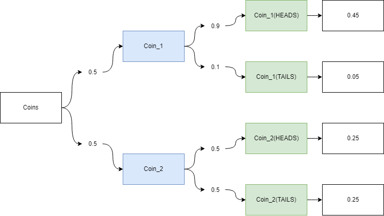
Two coins, one fair and other loaded.
- Coin 1: \(P_1(HEADS) = P_1(TAILS) = 0.5\);
- Coin 2: \(P_2(HEADS) = 0.9\) and \(P_2(TAILS) = 0.1\).

Figure 2
What is the probability of this sequence HEADS and TAILS?
| Coin | Flip 1 | Flip 2 | \(P_{coin}\) | \(P_{Flip 1}\) | \(P_{Flip 2}\) | P | Q2: HEADS then TAILS? | Q2: answer |
|---|---|---|---|---|---|---|---|---|
| 1 | H | H | 0.5 | 0.9 | 0.9 | 0.405 | No | 0 |
| 1 | H | T | 0.5 | 0.9 | 0.1 | 0.045 | Yes | 0.045 |
| 1 | T | H | 0.5 | 0.1 | 0.9 | 0.045 | No | 0 |
| 1 | T | T | 0.5 | 0.1 | 0.1 | 0.005 | No | 0 |
| 2 | H | H | 0.5 | 0.5 | 0.5 | 0.125 | No | 0 |
| 2 | H | T | 0.5 | 0.5 | 0.5 | 0.125 | Yes | 0.125 |
| 2 | T | H | 0.5 | 0.5 | 0.5 | 0.125 | No | 0 |
| 2 | T | T | 0.5 | 0.5 | 0.5 | 0.125 | No | 0 |
| \(SUM = 1\) | \(SUM = 0.170\) |
4.4.3.2 Summary
In this lesson you learned about conditional probability. Often events are not independent like with coin flips and dice rolling. Instead, the outcome of one event depends on an earlier event.
For example, the probability of obtaining a positive test result is dependent on whether or not you have a particular condition. If you have a condition, it is more likely that a test result is positive. We can formulate conditional probabilities for any two events in the following way:
- \(P(A|B) = \frac{P(A\text{ }\cap\text{ }B)}{P(B)}\)
- \(P(A ∩ B)\)
In this case, we could have this as:
\[P(positive|disease) = \frac{P(\text{positive }\cap\text{ disease})}{P(disease)}\]
where ∣ represents “given” and \(\cap\) represents “and”. — Class notes - Text: Summary
A work by AH Uyekita
anderson.uyekita[at]gmail.com