Chapter 6 GeomTimelineLabel
This geom_* performs the labels annotation on the geom_timeline plots.
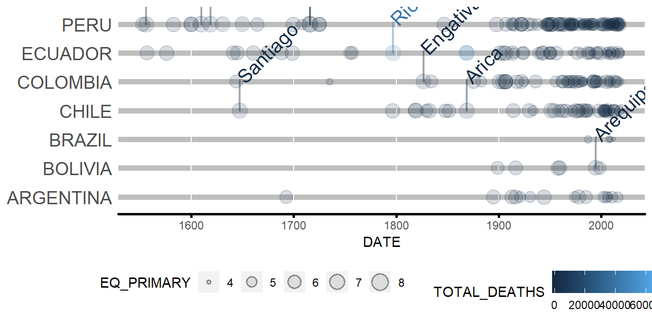
6.1 Example
Using ggplot2::layer to plot the visuals of GeomTimelineLabel.
# Path to the raw data.
raw_data_path <- system.file("extdata", "signif.txt", package = "msdr")

# Loading the dataset of Earthquake.
df <- readr::read_delim(file = raw_data_path,
                        delim = '\t',
                        col_names = TRUE,
                        progress = FALSE,
                        col_types = readr::cols())

# Cleaning and Creating LOCATION column.
df_clean <- df %>% eq_clean_data() %>% filter(COUNTRY %in% c('CHILE', 'COLOMBIA','ECUADOR',
                                                             'PERU', 'PARAGUAY','URUGUAY',
                                                             'BRAZIL', 'BOLIVIA', 'ARGENTINA'))

# Creating a simple geom_timeline plot.
simple_plot <- df_clean %>%
       ggplot2::ggplot() +
                     msdr::geom_timeline(aes(x = DATE,
                                             y = COUNTRY,
                                             size = EQ_PRIMARY,
                                             color = TOTAL_DEATHS))

# Adding the labels annotation using ggplot2::layer
simple_plot +
     ggplot2::layer(geom = GeomTimelineLabel,
                    mapping = aes(x     = DATE,
                                  label = LOCATION,
                                  y     = COUNTRY,
                                  mag   = EQ_PRIMARY,
                                  color = TOTAL_DEATHS,
                                  n_max = 10),
                    data = df_clean,
                    stat = 'identity',
                    position = 'identity',
                    show.legend = NA,
                    inherit.aes = TRUE,
                    params = list(na.rm = FALSE)) + theme_msdr()